Fick's laws of diffusion

For the technique of measuring cardiac output, see Fick principle.

Fick's laws of diffusion describe diffusion and can be used to solve for the diffusion coefficient, D. They were derived by Adolf Fick in the year 1855.

1 Fick's first law
2 Fick's second law
- 2.1 Example solution in one dimension: diffusion length
3 History
4 Applications
- 4.1 Biological perspective
5 Fick's flow in liquids
- 5.1 Semiconductor fabrication applications
6 Derivation of Fick's 1st law in 1 dimension
7 See also
8 Notes
9 References
10 External links

Fick's first law

Fick's first law relates the diffusive flux to the concentration, by postulating that the flux goes from regions of high concentration to regions of low concentration, with a magnitude that is proportional to the concentration gradient (spatial derivative). In one (spatial) dimension, this is

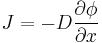
$\bigg. J = - D \frac{\partial \phi}{\partial x} \bigg.$

where

$J$ is the "diffusion flux" [(amount of substance) per unit area per unit time], example $(\tfrac{\mathrm{mol}}{ \mathrm m^2\cdot \mathrm s})$ . $J$ measures the amount of substance that will flow through a small area during a small time interval.

$\, D$ is the diffusion coefficient or diffusivity in dimensions of [length² time⁻¹], example $(\tfrac{\mathrm m^2}{\mathrm s})$

$\, \phi$ (for ideal mixtures) is the concentration in dimensions of [(amount of substance) length⁻³], example $(\tfrac\mathrm{mol}{\mathrm m^3})$

$\, x$ is the position [length], example $\,\mathrm m$

$\, D$ is proportional to the squared velocity of the diffusing particles, which depends on the temperature, viscosity of the fluid and the size of the particles according to the Stokes-Einstein relation. In dilute aqueous solutions the diffusion coefficients of most ions are similar and have values that at room temperature are in the range of 0.6x10⁻⁹ to 2x10⁻⁹ m²/s. For biological molecules the diffusion coefficients normally range from 10⁻¹¹ to 10⁻¹⁰ m²/s.

In two or more dimensions we must use $\nabla$ , the del or gradient operator, which generalises the first derivative, obtaining

$J=- D\nabla \phi$ .

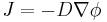The driving force for the one-dimensional diffusion is the quantity $- \frac{\partial \phi}{\partial x}$

which for ideal mixtures is the concentration gradient. In chemical systems other than ideal solutions or mixtures, the driving force for diffusion of each species is the gradient of chemical potential of this species. Then Fick's first law (one-dimensional case) can be written as:

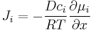
$J_i = - \frac{D c_i}{RT} \frac{\partial \mu_i}{\partial x}$

where the index i denotes the ith species, c is the concentration (mol/m³), R is the universal gas constant (J/(K mol)), T is the absolute temperature (K), and μ is the chemical potential (J/mol).

If the primary variable is mass fraction ( $y_i$ , given, for example, in $\tfrac{\mathrm kg}{\mathrm kg}$ ), then the equation changes to:

$J_i=- \rho D\nabla y_i$

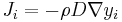
where $\rho$ is the fluid density (for example, in $\tfrac{\mathrm kg}{\mathrm m^3}$ ). Note that the density is outside the gradient operator.

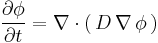
Fick's second law

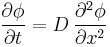
Fick's second law predicts how diffusion causes the concentration to change with time:

$\frac{\partial \phi}{\partial t} = D\,\frac{\partial^2 \phi}{\partial x^2}\,\!$

Where

$\,\phi$ is the concentration in dimensions of [(amount of substance) length⁻³], example $(\tfrac\mathrm{mol}{m^3})$
$\, t$ is time [s]
$\, D$ is the diffusion coefficient in dimensions of [length² time⁻¹], example $(\tfrac{m^2}{s})$
$\, x$ is the position [length], example $\,m$

It can be derived from Fick's First law and the mass balance:

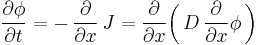
$\frac{\partial \phi}{\partial t} =-\,\frac{\partial}{\partial x}\,J = \frac{\partial}{\partial x}\bigg(\,D\,\frac{\partial}{\partial x}\phi\,\bigg)\,\!$

Assuming the diffusion coefficient D to be a constant we can exchange the orders of the differentiation and multiply by the constant:

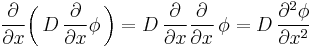
$\frac{\partial}{\partial x}\bigg(\,D\,\frac{\partial}{\partial x} \phi\,\bigg) = D\,\frac{\partial}{\partial x} \frac{\partial}{\partial x} \,\phi = D\,\frac{\partial^2\phi}{\partial x^2}$

and, thus, receive the form of the Fick's equations as was stated above.

For the case of diffusion in two or more dimensions Fick's Second Law becomes

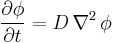$\frac{\partial \phi}{\partial t} = D\,\nabla^2\,\phi\,\!$ ,

which is analogous to the heat equation.

If the diffusion coefficient is not a constant, but depends upon the coordinate and/or concentration, Fick's Second Law yields

$\frac{\partial \phi}{\partial t} = \nabla \cdot (\,D\,\nabla\,\phi\,)\,\!$

An important example is the case where $\,\phi$ is at a steady state, i.e. the concentration does not change by time, so that the left part of the above equation is identically zero. In one dimension with constant $\, D$ , the solution for the concentration will be a linear change of concentrations along $\, x$ . In two or more dimensions we obtain

$\nabla^2\,\phi =0\!$

which is Laplace's equation, the solutions to which are called harmonic functions by mathematicians.

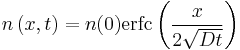
Example solution in one dimension: diffusion length

A simple case of diffusion with time t in one dimension (taken as the x-axis) from a boundary located at position $x=0$ , where the concentration is maintained at a value $n(0)$ is

$n \left(x,t \right)=n(0) \mathrm{erfc} \left( \frac{x}{2\sqrt{Dt}}\right)$ .

where erfc is the complementary error function. The length $2\sqrt{Dt}$ is called the diffusion length and provides a measure of how far the concentration has propagated in the x-direction by diffusion in time t.

As a quick approximation of the error function, the first 2 terms of the Taylor series can be used:

$n \left(x,t \right)=n(0) \left[ 1 - 2 \left(\frac{x}{2\sqrt{Dt\pi}}\right) \right]$

For more detail on diffusion length, see these examples.

History

In 1855, physiologist Adolf Fick first reported^[1]^[2] his now-well-known laws governing the transport of mass through diffusive means. Fick's work was inspired by the earlier experiments of Thomas Graham, but which fell short of proposing the fundamental laws for which Fick would become famous. The Fick's law is analogous to the relationships discovered at the same epoch by other eminent scientists: Darcy's law (hydraulic flow), Ohm's law (charge transport), and Fourier's Law (heat transport).

Fick's experiments (modeled on Graham's) dealt with measuring the concentrations and fluxes of salt, diffusing between two reservoirs through tubes of water. It is notable that Fick's work primarily concerned diffusion in fluids, because at the time, diffusion in solids was not considered generally possible.^[3] Today, Fick's Laws form the core of our understanding of diffusion in solids, liquids, and gases (in the absence of bulk fluid motion in the latter two cases). When a diffusion process does not follow Fick's laws (which does happen), we refer to such processes as non-Fickian, in that they are exceptions that "prove" the importance of the general rules that Fick outlined in 1855.

Applications

Equations based on Fick's law have been commonly used to model transport processes in foods, neurons, biopolymers, pharmaceuticals, porous soils, population dynamics, semiconductor doping process, etc. Theory of all voltammetric methods is based on solutions of Fick's equation. A large amount of experimental research in polymer science and food science has shown that a more general approach is required to describe transport of components in materials undergoing glass transition. In the vicinity of glass transition the flow behavior becomes "non-Fickian". See also non-diagonal coupled transport processes (Onsager relationship).

Biological perspective

The first law gives rise to the following formula:^[4]

$\text{Flux} = {-P\cdot A\cdot (c_2 - c_1)}\,\!$

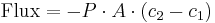
in which,

$\, P$ is the permeability, an experimentally determined membrane "conductance" for a given gas at a given temperature.
$\, A$ is the surface area over which diffusion is taking place.
$\, c_2 - c_1$ is the difference in concentration of the gas across the membrane for the direction of flow (from $c_1$ to $c_2$ ).

Fick's first law is also important in radiation transfer equations. However, in this context it becomes inaccurate when the diffusion constant is low and the radiation becomes limited by the speed of light rather than by the resistance of the material the radiation is flowing through. In this situation, one can use a flux limiter.

The exchange rate of a gas across a fluid membrane can be determined by using this law together with Graham's law.

Fick's flow in liquids

When two miscible liquids are brought into contact, and diffusion takes place, the macroscopic (or average) concentration evolves following Fick's law. On a mesoscopic scale, that is, between the macroscopic scale described by Fick's law and molecular scale, where molecular random walks take place, fluctuations cannot be neglected. Such situations can be successfully modeled with Landau-Lifshitz fluctuating hydrodynamics. In this theoretical framework, diffusion is due to fluctuations whose dimensions range from the molecular scale to the macroscopic scale. ^[5]

In particular, fluctuating hydrodynamic equations include a Fick's flow term, with a given diffusion coefficient, along with hydrodynamics equations and stochastic terms describing fluctuations. When calculating the fluctuations with a perturbative approach, the zero order approximation is Fick's law. The first order gives the fluctuations, and it comes out that fluctuations contribute to diffusion. This represents somehow a tautology, since the phenomena described by a lower order approximation is the result of a higher approximation: this problem is solved only by renormalizing fluctuating hydrodynamics equations.

Semiconductor fabrication applications

IC Fabrication technologies, model processes like CVD, Thermal Oxidation, and Wet Oxidation, doping, etc. use diffusion equations obtained from Fick's law.

In certain cases, the solutions are obtained for boundary conditions such as constant source concentration diffusion, limited source concentration, or moving boundary diffusion (where junction depth keeps moving into the substrate).

Derivation of Fick's 1st law in 1 dimension

The following derivation is based on a similar argument made in Berg 1977 (see references).

Consider a collection of particles performing a random walk in one dimension with length scale $\Delta x$ and time scale $\Delta t$ . Let $N(x, t)$ be the number of particles at position $x$ at time $t$ .

At a given time step, half of the particles would move left and half would move right. Since half of the particles at point $x$ move right and half of the particles at point $x %2B \Delta x$ move left, the net movement to the right is:

$-\frac{1}{2}\left[N(x %2B \Delta x, t) - N(x, t)\right]$

The flux, J, is this net movement of particles across some region normal to the random walk during a time interval, $\Delta t$ . Hence we may write:

$J = - \frac{1}{2} \left[\frac{ N(x %2B \Delta x, t)}{a \Delta t} - \frac{ N(x, t)}{a \Delta t}\right]$

Multiplying the top and bottom of the righthand side by $(\Delta x)^2$ and rewriting, we obtain:

$J = -\frac{\left(\Delta x\right)^2}{2 \Delta t}\left[\frac{N(x %2B \Delta x, t)}{a (\Delta x)^2} - \frac{N(x, t)}{a (\Delta x)^2}\right]$

We note that concentration is defined as particles per unit volume, and hence 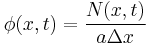$\phi (x, t) = \frac{N(x, t)}{a \Delta x}$ .

In addition, $-\tfrac{\left(\Delta x\right)^2}{2 \Delta t}$ is the definition of the diffusion constant in one dimension, $D$ . Thus our expression simplifies to:

$J = -D \left[\frac{\phi (x %2B \Delta x, t)}{\Delta x} - \frac{\phi (x , t)}{\Delta x}\right]$

In the limit where $\Delta x$ is infinitesimal, the righthand side becomes a space derivative:

References

- W.F. Smith, Foundations of Materials Science and Engineering 3rd ed., McGraw-Hill (2004)
- H.C. Berg, Random Walks in Biology, Princeton (1977)